The Oracle’s Automatic Workload Repository (AWR) collects, processes, and maintains performance statistics for problem detection and self-tuning purposes. The report generated by AWR is a big report and it can take years of experience to actually understand all aspects of this report. In this post we will try to explain some important sections of AWR, significance of those sections and also some important tips. Please note that explaining all sections of AWR will not be possible so we will stick to some of the most frequently used sections.
Note that this is not comprehensive information and goal is to help in giving an overview of few key sections to Junior DBAs as a primer and to encourage them to build further the knowledge in related fields.
To start with let us mention some high level important tips regarding AWR:
1. Collect Multiple AWR Reports: It’s beneficial to have two AWR Reports, one for the good time and other when performance is poor or you can create three reports (Before/Meantime/After reports) during the time frame problem was experienced and compare it with the time frame before and after.
2. Stick to Particular Time: You must have a specific time when Database was slow so that you can choose a shorter timeframe to get a more precise report.
3. Split Large AWR Report into Smaller Reports: Instead of having one report for long time like one report for 3 hrs. it is better to have three reports each for one hour. This will help to isolate the problem
4. FOR RAC, take each instance’s individual report: For RAC environment, you need to do it separately of all the instances in the RAC to see if all the instances are balanced the way they should be.
5. Use ASH also : Use AWR to identify the troublesome areas and then use ASH to confirm those areas.
6. Increase the retention period : Some instances where you get more performance issues you should increase the retention time so that you can have historical data to compare.
TIME UNITS USED IN VARIOUS SECTIONS OF AWR REPORTS
-> s – second
-> cs – centisecond – 100th of a second
-> ms – millisecond – 1000th of a second
-> us – microsecond – 1000000th of a second
Top Header
SIGNIFICANCE OF THIS SECTION:
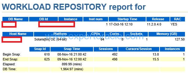
This contains information about the Database and environment. Along with the snapshot Ids and times. Important thing to notice is that the configuration like CPU and Memory has not changed when the performance is degraded.
| PARAMETER | DESCRIPTION | ANALYSIS |
| DB TIME | Time spent in database during the Elapsed Time OR Sum of the time taken by all sessions in the database during the ‘Elapsed’ time.DB Time= CPU Time + Non IDLE wait time. Note: it does not include background processes |
DB TIME > Elapsed Time will mean that the sessions were active on database concurrently
You cam find the average active sessions during AWR Time: DB TIME/ELAPSED => 1964.97/899.99 = 2.18 So database load (average active sessions) = 2.18 (SAME IDEA AS CPU LOAD on UNIX) It means that May be ~2 users were active on database for ‘Elapsed’ Time. If DB Time has higher value means DB Activity/Sessions were High during the AWR Time. AWR REPORT THAT WE WILL REVIEW BELOW IS BASED ON THIS DB TIME. This means that for every minute of Elapsed time there is 2.2 minutes of work in done in the database
|
| ELAPSED TIME | The time duration in which this AWR report has been generated. |
Elapsed time should contain the issue duration. Take manual snapshots if required |
| CPUs | Thread count per core. It is not “actual” CPU. | |
| STARTUP TIME | Database startup time | |
| RAC | If you have more than one node then take AWR from all nodes if you don’t know issues are happening in which node. |
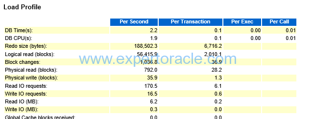
Here in load profile (average active sessions, DB CPU, logical and physical reads, user calls, executions, parses, hard parses, logons, rollbacks, transactions) —
check if the numbers are consistent with each other and with general database profile (OLTP/DWH/mixed)
- Pay most attention to physical reads, physical writes, hard parse to parse ratio and executes to transaction ratio.
- The ratio of hard parses to parses tells you how often SQL is being fully parsed. Full parsing of SQL statements has a negative effect on performance.
- High hard parse ratios (>2 – 3 percent) indicate probable bind variable issues or maybe versioning problems.
- Rows per sort can also be reviewed here to see if large sorts are occurring.
- This section can help in the load testing for application releases. You can compare this section for the baseline as well as high load situation.
| PARAMETER | DESCRIPTION | ANALYSIS |
| Redo Size (Bytes) | The main sources of redo are (in roughly descending order): INSERT, UPDATE and DELETE. For INSERTs and UPDATE s | Not very scary number in our report
High redo figures mean that either lots of new data is being saved into the database, or existing data is undergoing lots of changes. What do you do if you find that redo generation is too high (and there is no business reason for that)? Not much really — since there is no “SQL ordered by redo” in the AWR report. Just keep an eye open for any suspicious DML activity. Any unusual statements? Or usual statements processed more usual than often? Or produce more rows per execution than usual? Also, be sure to take a good look in the segments statistics section (segments by physical writes, segments by DB block changes etc.) to see if there are any clues there. |
| DB CPU | Its the amount of CPU time spent on user calls. Same as DB time it does not include background process. The value is in microseconds | We have 8 CORES and so we can potentially use 8 seconds of CPU time per second. In this case DB CPU (s) : 1.9 (per second) is reporting that the system is using 1.9 seconds of CPU of the potential 8 seconds/second that it can use.We are not CPU Bound |
| LOGICAL READS | Consistent gets + db block gets = Logical Reads
As a process, Oracle will try to see if the data is available in Buffer cache i.e. SGA? If it does, then logical read increases to 1. To explain a bit further, if Oracle gets the data in a block which is consistent with a given point in time, then a counter name “Consistent Gets” increases to 1. But if the data is found in current mode, that is, the most up-to-date copy of the data in that block, as it is right now or currently then it increases a different counter name “db block Gets”. Therefore, a Logical read is calculated as = Total number of “Consistent Gets” + Total number of “db block gets”. These two specific values can be observed in ‘Instance Activity Stats’ section. |
Logical and physical reads combined shows measure of how many IO’s (Physical and logical) that the database is performing..
If this is high go to section “SQL by logical reads”. That may help in pointing which SQL is having more logical reads. |
| USER QUERIES | Number of user queries generated | |
| PARSES | The total of all parses, hard and soft | |
| HARD PARSES | The parses requiring a completely new parse of the SQL statement. These consume both latches and shared pool area. | How much hard parsing is acceptable?
It depends on too many things, like number of CPUs, number of executions, how sensitive are plans to SQL parameters etc. But as a rule of a thumb, anything below 1 hard parse per second is probably okay, and everything above 100 per second suggests a problem (if the database has a large number of CPUs, say, above 100, those numbers should be scaled up accordingly). It also helps to look at the number of hard parses as % of executions (especially if you’re in the grey zone). If you suspect that excessive parsing is hurting your database’s performance: 1) check “time model statistics” section (hard parse elapsed time, parse time elapsed etc.) 2) see if there are any signs of library cache contention in the top-5 events 3) see if CPU is an issue. |
| Soft Parses: | Soft parses are not listed but derived by subtracting the hard parses from parses. A soft parse reuses a previous hard parse; hence it consumes far fewer resources. | |
| Physical Reads | But if it Oracle does not find the data in buffer cache, then it reads it from physical block and increases then Physical read count to 1. Clearly, buffer get is less expensive than physical read because database has to work harder (and more) to get the data. Basically time it would have taken if available in buffer cache + time actually taken to find out from physical block. | If this is high go to section “SQL by Physical reads”. That may help in pointing which SQL is having more Physical reads. |
| Executes (SQL) | If executes per second looks enormous then its a red flag.
Example: This numbers, combined with high CPU usage, are enough to suspect there MAY BE context switching as the primary suspect: a SQL statement containing a PL/SQL function, which executes a SQL statement hundreds of thousands of time per function call. if it is high then it also suggests that most of the database load falls on SQL statements in PL/SQL routines. |
|
| User Calls | number of calls from a user process into the database – things like “parse”, “fetch”, “execute”, “close” | This is an extremely useful piece of information, because it sets the scale for other statistics (such as commits, hard parses etc.).
In particular, when the database is executing many times per a user call, this could be an indication of excessive context switching (e.g. a PL/SQL function in a SQL statement called too often because of a bad plan). In such cases looking into “SQL ordered by executions” will be the logical next step. |
| Logons | logons – really means what it means. Number of logons | Establishing a new database connection is also expensive (and even more expensive in case of audit or triggers). “Logon storms” are known to create very serious performance problems. If you suspect that high number of logons is degrading your performance, check “connection management elapsed time” in “Time model statistics”. |
Sorts |
Sort operations consume resources. Also, expensive sorts may cause your SQL fail because of running out of TEMP space. So obviously, the less you sort, the better (and when you do, you should sort in memory). However, I personally rarely find sort statistics particularly useful: normally, if expensive sorts are hurting your SQL’s performance, you’ll notice it elsewhere first. | |
| DB Time | average number of active sessions is simply DB time per second. | |
| Block Changes | Number of blocks modified during the sample interval |
Instance Efficiency Percentage
| PARAMETER | DESCRIPTION | ANALYSIS |
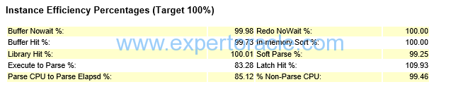
| In memory sort % | Shows %of times Sorting operations happened in memory than in the disk (temporary tablespace). | In Memory Sort being low (in the high 90s or lower) indicates PGA_AGGREGATE_TARGET or SORT_AREA_SIZE issues |
| soft parse % | Shows % of times the SQL in shared pool is used. Shows how often sessions issued a SQL statement that is already in the shared pool and how it can use an existing version of that statement. | Soft Parsing being low indicates bind variable and versioning issues. With 99.25 % for the soft parse meaning that about 0.75 % (100 – soft parse) is happening for hard parsing. Low hard parse is good for us. |
| % Non-Parse CPU | Oracle utilizes the CPU mostly for statement execution but not for parsing. | If this value is near 100% means most of the CPU resources are used into operations other than parsing, which is good for database health.
Most of our statements were already parsed so we weren’t doing a lot of re parsing. Re parsing is high on CPU and should be avoided. |
| Execute to Parse % | Shows how often parsed SQL statements are reused without re-parsing. | The way this ratio is computed, it will be a number near 100 percent when the application executes a given SQL statement many times over but has parsed it only once.
If the number of parse calls is near the number of execute calls, this ratio trends towards zero. If the number of executes increase while parse calls remain the same this ratio trends up. When this number is low, parsing is consuming CPU and shared pool latching. |
| Parse CPU to Parse Elapsed % | Gives the ratio of CPU time spent to parse SQL statements. | If the value are low then it means that there could be a parsing problem. You may need to look at bind variable issues or shared pool sizing issue. If low it also means some bottleneck is there related to parsing. We would start by reviewing library cache contention and contention in shared pool latches. You may need to increase the shared pool. |
| Buffer Hit % | Measures how many times a required block was found in memory rather than having to execute an expensive read operation on disk to get the block. | |
| Buffer Nowait% | Indicates % of times data buffers were accessed directly without any wait time. | This ratio relates to requests that a server process makes for a specific buffer. This is the percentage of those requests in which the requested buffer is immediately available. All buffer types are included in this statistic. If the ratio is low, check the Buffer Wait Statistics section of the report for more detail on which type of block is being contended. Most likely, additional RAM will be required. |
| Library Hit% | Shows % of times SQL and PL/SQL found in shared pool. | Library hit % is great when it is near 100%. If this was under 95% we would investigate the size of the shared pool.
In this ration is low then we may need to: |
| Latch Hit % | Shows % of time latches are acquired without having to wait. | If Latch Hit % is <99%, you may have a latch problem. Tune latches to reduce cache contention |
| Redo NOWait% | Shows whether the redo log buffer has sufficient size. |
Top 10 Foreground Wait Events by Total Wait Time
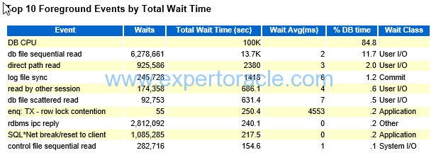
Note that there could be significant waits that are not listed here, so check the Foreground Wait Events (Wait Event Statistics) section for any other time consuming wait events.
For the largest waits look at the Wait Event Histogram to identify the distribution of waits.
| PARAMETER | DESCRIPTION | ANALYSIS |
| DB CPU | Time running in CPU (waiting in run-queue not included) |
Here 84.8% is the %DB Time for this Event which is really HIGH!
DB Time was 1965 minutes and DB CPU is (100000/60= 1667 minutes) We can find 1) DB CPU LOAD =Total wait time /AWR TIME 2) DB CPU UTLIZATION % IMPORTANT: Your server may have other database instances sharing the CPU resources so take into account those too. Also this do not mean that server CPU is 84% Utilized!
|
| Sum of %DB Time | The sum should be approx 100%. If it is way below 100% then it may mean that wait events were irrelevant OR Server is overloaded. | |
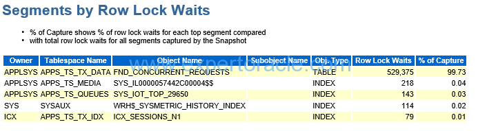
| enq TX – row lock contention | waited for locked rows | This parameter value currently is only 0.2% of total DB time so we don’t have to much worry about it.
Say that it was higher value, 10% then we will have to look into root cause. You will have to go to “Segments by Row Lock Waits” and see what tables are getting locked and then you will have to see in which SQL_ID these are used.
|
| DB FILE SEQUENTIAL READ | single block i/o
Sequential read is an index read followed by table read because it is doing index lookups which tells exactly which block to go to
|
Average I/O call is 2ms which is not very high. If you have say very high wait average example 100ms or 200ms, it means that your disks are slow
Are your SQLs returning too many rows, is the I/O response pretty bad on the server, is DB not sized to cache enough result sets You need to see then the “File IO Stats” section in the AWR report. The event indicates that index scan is happening while reading data from table. High no. of such event may be a cause of unselective indexes i.e. oracle optimizer is not selecting proper indexes from set of available indexes. This will result in extra IO activity and will contribute to delay in SQL execution. Generally high no. is possible for properly tuned application having high transaction activity. •If Index Range scans are involved, more blocks than necessary could be being visited if the index is un-selective.By forcing or enabling the use of a more selective index, we can access the same table data by visiting fewer index blocks (and doing fewer physical I/Os). •If indexes are fragmented, we have to visit more blocks because there is less index data per block. In this case, re-building the index will compact its contents into fewer blocks. • If the index being used has a large Clustering Factor, then more table data blocks have to be visited in order to get the rows in each index block. By rebuilding the table with its rows sorted by the particular index columns we can reduce the Clustering Factor and hence the number of table data blocks that we have to visit for each index block.
|
| LOG FILE SYNC | Here Wait AVG (MS) is 6 which is not a cry number. Above 20ms we don’t consider good numberAlso go to “Instance Activity Stats” section and see how many commits actually happened and then see here that what % of COMMITS have to wait.Remember that short transactions, frequent commits is property of OLTP Application. |
|
| DB FILE SCATTERED READ | caused due to full table scans may be because of insufficient indexes or un-avilablity of updated statistics | To avoid this event, identify all the tables on which FTS is happening and create proper indexes so that oracle will do Index scans instead of FTS. The index scan will help in reducing no. of IO operations.
To get an idea about tables on which FTS is happening please refer to “Segment Statistics” -> “Segments By Physical Read” section of AWR report. This section lists down both Tables and Indexes on which Physical Reads are happening. Please note that physical reads doesn’t necessarily means FTS but a possibility of FTS. |
| Concurrency, wait class | Concurrency wait class is not good and if high then need to be analyzed. | |
| direct path read temp or direct path write temp | this wait event shows Temp file activity (sort,hashes,temp tables, bitmap) check pga parameter or sort area or hash area parameters. You might want to increase them |
|
| Wait Class, column | helps in classifying whether the issue is related to application or infrastructure. | Wait events are broadly classified in to different WAIT CLASSES:
Administrative |
| Buffer Busy Wait | Indicates that particular block is being used by more than one processes at the same. When first process is reading the block the other processes goes in a wait as the block is in unshared more. Typical scenario for this event to occur is, when we have batch process which is continuously polling database by executing particular SQL repeatedly and there are more than one parallel instances running for the process. All the instances of the process will try to access same memory blocks as the SQL they are executing is the same. This is one of the situation in which we experience this event. | |
| enq: TX – row lock contention: | Oracle maintenance data consistency with the help of locking mechanism. When a particular row is being modified by the process, either through Update/ Delete or Insert operation, oracle tries to acquire lock on that row. Only when the process has acquired lock the process can modify the row otherwise the process waits for the lock. This wait situation triggers this event. The lock is released whenever a COMMIT is issued by the process which has acquired lock for the row. Once the lock is released, processes waiting on this event can acquire lock on the row and perform DML operation. | |
| enq: UL – contention: | This enq wait occurs when application explicitly locks by executing the lock table command. | |
| enq: TM – contention | This usually happens due to a missing foreign key constraint on a table that’s part of a DML operation. |
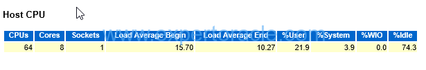
Host CPU
| PARAMETER | DESCRIPTION | ANALYSIS |
| CPUs | are actually threads. Here we have 8 Cores and 8 Threads per Core so CPU = number of core X number of threads per core = 8 X 8 = 64 |
|
| Load Average | Compare Load average with Cores.
Very Ideal thing is that Load Average should be less than Cores although this may not be happening (any it may not be issue also!) |
|
| %Idle | Can be misleading as sometimes your %Idle can be 50% but your server is starving for CPU.
50% means that all your cores are BUSY. You may have free threads (CPU) but you can not run two processes CONCURRENTLY on same CORE. All % in this reports are calculated based on CPU ( which are actually threads)
|
|
| Cores | Here we have 8 core system So we have 8 cores, meaning in a 60 min hour we have 60 X 8 = 480 CPU minsand total AWR duration is 8 hoursso 480X8 = 3840 CPU minutes in total |
Instance CPU
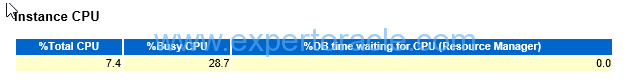
SIGNIFICANCE OF THIS SECTION:
A high level of DB CPU usage in the Top N Foreground Events (or Instance CPU: %Busy CPU) does not necessarily mean that CPU is a bottleneck. In this example also we have DB CPU as the highest consuming category in the “Top 10 Foreground Events”
Look at the Host CPU and Instance CPU sections. The key things to look for are the values “%Idle” in the “Host CPU” section and “%Total CPU” in the “Instance CPU” section.
If the “%Idle” is low and “%Total CPU” is high then the instance could have a bottleneck in CPU (be CPU constrained). Otherwise, the high DB CPU usage just means that the database is spending a lot of time in CPU (processing) compared to I/O and other events. In either case (CPU is a bottleneck or not) there could be individual expensive SQLs with high CPU time, which could indicate suboptimal
execution plans, especially if accompanied with high (buffer) gets.
If you see in our case %idle is high 74% AND %Total CPU is just 7.45 so CPU is not a bottle neck in this example.
Cache Sizes
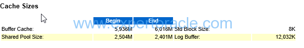
SIGNIFICANCE OF THIS SECTION:
From Oracle 10g onwards, database server does Automatic Memory Management for PGA and SGA components. Based on load, database server keeps on allocating or deallocating memory assigned to different components of SGA and PGA. Due to this reason, we can observe different sizes for Buffer Cache and Shared Pool, at the beginning or end of AWR snapshot period.
Shared Pool Statistics
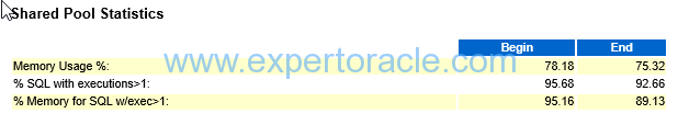
| PARAMETER | DESCRIPTION | ANALYSIS |
| Memory Usage% | shared pool usage |
If your usage is low (<85 percent) then your shared pool is over sized. if Memory Usage % is too large like 90 % it could mean that your shared pool is tool small |
| % SQL with executions >1 | Shows % of SQLs executed more than 1 time. The % should be very near to value 100. | If your reuse is low (<60 – 70 percent) you may have bind variable or versioning issues. Ideally all the percentages in this area of the report should be as high (close to 100) as possible. |
| memory for SQL w/exec>1 | From the memory space allocated to cursors, shows which % has been used by cursors more than 1. |
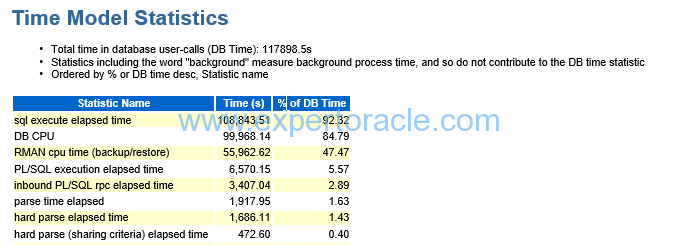
Time Model Statistics
|
SIGNIFICANCE OF THIS SECTION:
Important statistics here is the DB Time. The statistic represents total time spent in database calls. It is calculated by aggregating the CPU time and wait time of all sessions not waiting on idle event (non-idle user sessions). Since this timing is cumulative time for all non-idle sessions, it is possible that the time will exceed the actual wall clock time.
|
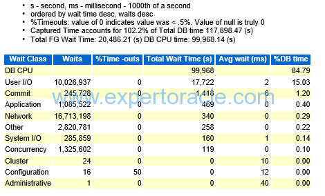
Foreground Wait Class
| PARAMETER | DESCRIPTION | ANALYSIS |
| User I/O | High User IO means,
From the pool of available indexes proper indexes are not being used |
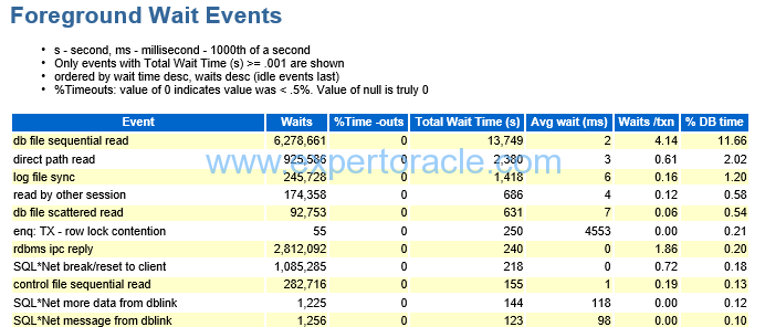
Foreground Wait Events
| PARAMETER | DESCRIPTION | ANALYSIS |
| SQL*Net Message from client | Idle wait event |
We can find the number of average inactive sessions by this wait event
Number of inactive sessions = 12679570/ (900 * 60) = 235 average inactive sessions This doesn’t mean user sessions as such but the number of such connections from Application Server connection pool.
|
| Direct path read/write to temp | Shows excessive sorting/hashing/global temp table/bitmap activity going to your temporary tablespace. Review PGA_AGGREGATE_TARGET settings. Even if it looks like it is big enough, if you aregetting multiple small sorts to disk it could mean your user load is over-utilizing it. | |
| SQL*Net Message to client | SQL*Net message to client waits almost always indicates network contention. | |
| SQL*Net more data from client | If it is very low then it indicates that the Oracle Net session data unit size is likely set correctly. | |
| Db file sequential reads | Usually indicates memory starvation, look at the db cache analysis and for buffer busy waits along with cache latch issues. | |
| Db file scattered reads | Usually indicates excessive full table scans, look at the AWR segment statistics for tables that are fully scanned | |
| Log file Sync | Log file related waits: Look at excessive log switches, excessive commits or slow IO subsystems. |
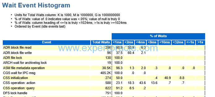
Wait Event Histogram
| PARAMETER | DESCRIPTION | ANALYSIS |
| DB FILE SEQUENTIAL READ | This parameter will have mostly higher number of wait events in the histogram.
Now if you see approx 50% wait events have less than 1 ms of wait and another 30% has less than 2 ms. It means that our disks are working good. Wait is low for most of the sessions going to database. We simply don’t want that high% (and high wait events numbers) are above 8ms of wait. Now if you see that the DB FILE SEQUENTIAL READ is the key wait event then next thing will be to find a) which segment is the bottleneck (go to “Segments by Physical Reads” section
|
SQL ordered by Elapsed Time
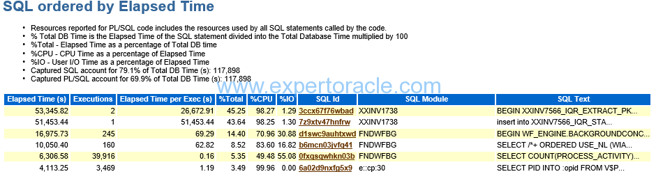
In this report, look for query has low executions and high Elapsed time per Exec (s) and this query could be a candidate for troubleshooting or optimizations. In above report, you can see first query has maximum Elapsed time but only 2 execution. So you have to investigate this.
| PARAMETER | DESCRIPTION | ANALYSIS |
| Elapse per Exec (s) | Elapse time in seconds for per execution of the SQL. | |
| Captured SQL Account for 79.1% of total DB Time |
Shows that how many % of SQL this AWR report was able to capture and show us | Remember that AWR reports shows those SQL which were in shared pool at the end of the AWR Time.
This number should be high value which will mean that we were able to capture all those SQLs which consumed the DB Time. If this is low number than try to generate AWR for lower snap duration so that we are able to capture the required SQLs which are consuming DB Time
|
| Executions | Total no. of executions for the SQL during the two snapshot period. An important point, if executions is 0 also sometimes, it doesn’t means query is not executing, this might be the case when query was still executing and you took AWR report. That’s why query completion was not covered in Report. |
|
| SQL Module | Provides module detail which is executing the SQL. Process name at the OS level is displayed as SQL Module name.
If the module name starts with any of the names given below, then don’t consider these SQLs for tuning purpose as these SQLs are oracle internal SQLs, DBMS, In the list XXIN1768 has two SQLIDs. The SQL id #1 is PL/SQL code as a wrapper and it took around 53k seconds. The sql #2 took 51k seconds and seems to be called in sql ID# 1, as their module names are same. Since the SQL#2 insert statement took almost all of the time so we sill focus on this query for tuning. |
|
| Elasped Time | The Elapsed Time is the sum of all individual execution time for the sql_id. So if multiple sessions execute the same SQLs, the elapsed time can be greater than the period of two snap_ids. |
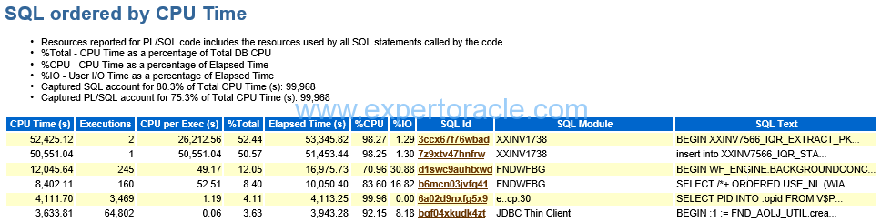
SQL ordered by CPU Time
| PARAMETER | DESCRIPTION | ANALYSIS |
| The top record in this table | The first and second report are part of same transaction. Second SQL is the inside part of first PLSQL.It is accounting huge % of the DB CPU and remember that DB CPU was the top event in our AWR. |
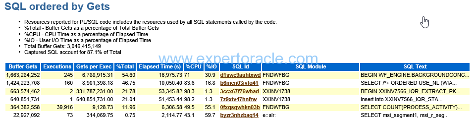
SQL ordered by Gets
| PARAMETER | DESCRIPTION | ANALYSIS |
| Gets per Exec | HOW MANY BLOCKS WERE READ | insert statement in XXINV1738 module has Gets per Exec that is too high, you need to analyze the SQL with some additional output such as sqlt and sqlhc. |
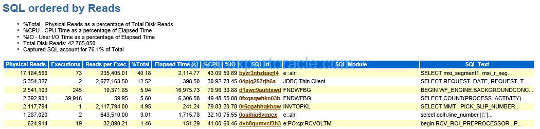
SQL ordered by Reads
| PARAMETER | DESCRIPTION | ANALYSIS |
| Captured SQL account for 76% of total | Our goal is to have this % as high as possible. Probably breaking down this AWR into smaller interval will increase this %.
|
|
| The top record in this table | We have seen in the “Segments by Physical Reads” section that MTL_ITEM_CATEGORIES account for 51.32% and looking here the SQL_ID which is a top and having 40.18% TOTAL is using this table.Yousee here that although it has executed 73 times but reads per executions is high making it top query consuming physical i/o.In contrast query at number 4 in this table has been executed around 40k times but since reads per execution is low so number 4th query is not the top query to worry about. |
|
| Reads per Exec | Possible reasons for high Reads per Exec are use of unselective indexes require large numbers of blocks to be fetched where such blocks are not cached well in the buffer cache, index fragmentation, large Clustering Factor in index etc. |
SQL ordered by Physical Reads (UnOptimized)
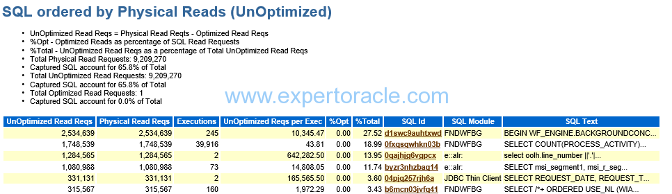
| PARAMETER | DESCRIPTION | ANALYSIS |
| Physica Read Reqs | Note that the ‘Physical Read Reqs’ column in the ‘SQL ordered by Physical Reads (UnOptimized)’ section is the number of I/O requests and not the number of blocks returned. Be careful not to confuse these with the Physical Reads statistics from the AWR section ‘SQL ordered by Reads’, which counts database blocks read from the disk not actual I/Os (a single I/O operation may return many blocks from disk). |
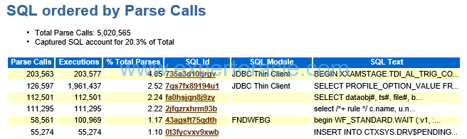
SQL ordered by Parse Calls
Tablespace IO Stats
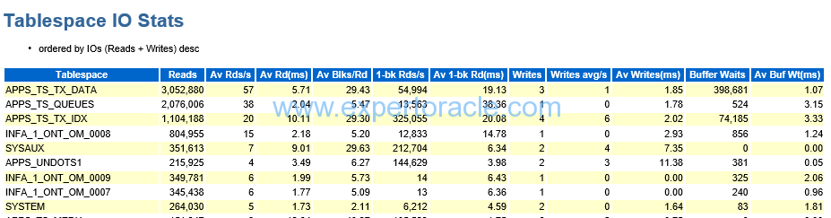
| PARAMETER | DESCRIPTION | ANALYSIS |
| Av Rd(ms) | Av Rd(ms) on the tablespace IO stats should be controlled under 10, which is ideal. But Avg read (ms) of up to 20 is acceptable for IO performance.
NOTE: When the figure in Reads column is too low, you can ignore the Av Rd(ms).
|
|
| Av Buf Wt(ms | Av Buf Wt(ms) on the tablespace IO stats should be controlled under 10, which is ideal. |
Buffer Pool Advisory
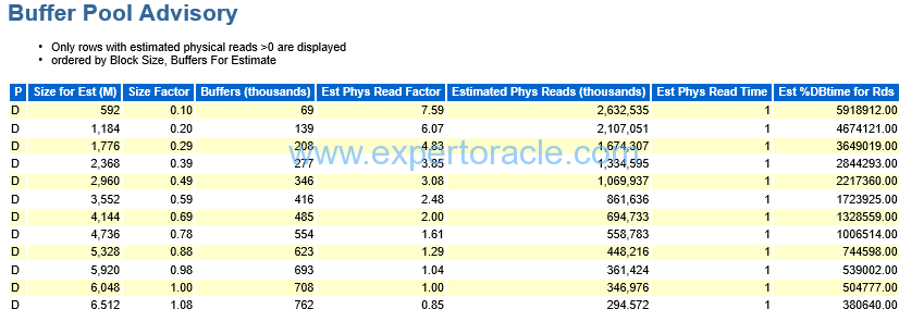
| PARAMETER | DESCRIPTION | ANALYSIS |
| First Parameter “P” | Apart from default buffer cache – pool (or subpool) which is always present, buffer cache may have other subpools.
Buffer Cache Advisory section will then have separate subsection for each of those subpools distinguished from others by a letter in the very left column of the section as follows: |
|
| Size Factor | Changing ‘Size Factor’ shows ratio of the proposed size of the buffer cache (increased or decreased) to the approximate actual size currently in use found in the row with ‘Size Factor’ = 1.0. | |
| Estimated Phys Read Factor | Changing ‘Estimated Phys Read Factor’ shows ratio of the estimated number of Physical Reads for the proposed (increased or decreased) size of the buffer cache to the number of Physical Reads calculated for the current size of buffer cache found in the row with ‘Estimated Phys Read Factor’ = 1.0. | HERE WE CAN SEE THAT IF WE INCREASE OUR BUFFER CACHE FROM 6 GB TO 10 GB IT IS HELPING US SIGNIFICANTLY
THIS FACTOR WILL COME DOWN FROM 1 TO 0.3. |
PGA Memory Advisory
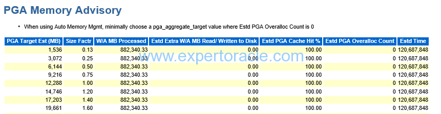
| PARAMETER | DESCRIPTION | ANALYSIS |
| Estd PGA Overalloc Count | Shows how many times the database instance processes would need to request more PGA memory at the OS level than the amount shown in the ‘PGA Target Est (MB)’ value of the respective row. Ideally this field should be 0 (indicating that the PGA is correctly sized, and no overallocations should take place), and that is your equally important second goal. In the given example this goal is achieved with PGA_AGGREGATE_TARGET of even 1,536MB.
So our PGA allocation is way too high. |
Shared Pool Advisory
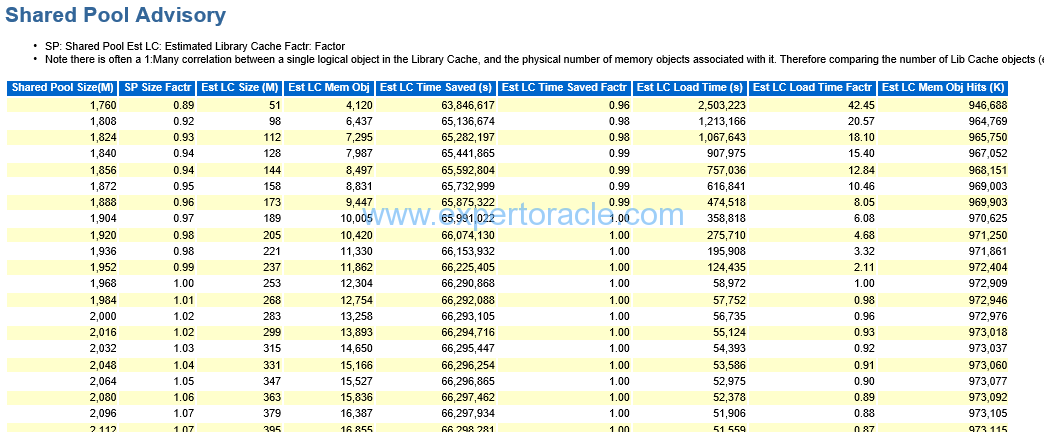
| PARAMETER | DESCRIPTION | ANALYSIS |
| EST LC TIME SAVED | LC means LIBRARY CACHE |
you have to see that if increase your shared pool then what is the amount of this time that you can save |
SGA Target Advisory
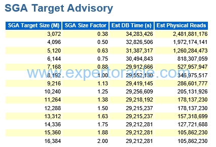
SIGNIFICANCE OF THIS SECTION:
The SGA target advisory report is somewhat of a summation of all the advisory reports previously presented in the AWR report. It helps you determine the impact of changing the settings of the SGA target size in terms of overall database performance. The report uses a value called DB Time as a measure of the increase or decrease in performance relative to the memory change made. Also the report will summarize an estimate of physical reads associated with the listed setting for the SGA.
Starting at a “Size Factor” of 1 (this indicates the current size of the SGA). If the “Est DB Time (s)” decreases significantly as the “Size Factor” increases then increasing the SGA will significantly reduce the physical reads and improve performance. but here in our example the Est DB Time is not reducing as much with increase in SGA so increasing SGA in our case will not be beneficial.
When the SQL requires a large volume of data access, increasing the SGA_TARGET size can reduce the amount of disk I/O and improve the SQL performance.
Buffer Wait Statistics
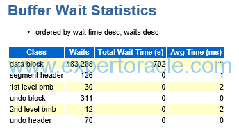
SIGNIFICANCE OF THIS SECTION:
The buffer wait statistics report helps you drill down on specific buffer wait events, and where the waits are occurring
We focus on Total wait time(s) and in this example this value is only 702 seconds
Avg time(ms) is also only 1 ms
Enqueue Activities
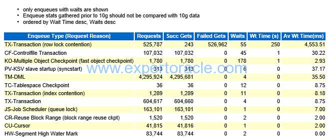
The Enqueue activity report provides information on enqueues (higher level Oracle locking) that occur. As with other reports, if you see high levels of wait times in these reports, you might dig further into the nature of the enqueue and determine the cause of the delays.
This can give some more information for enqueue waits (e.g. Requests, Successful gets, Failed gets), which can give an indication of the percentage of times that an enqueue has to wait and the number of failed gets.
In our example the top row do have failed gets but the number of waits is only 55 and wait time (s) is also not high number. So Enqueue is not our major issue in this AWR.
Undo Segment Summary
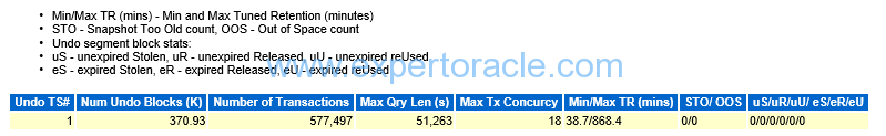
| PARAMETER | DESCRIPTION | ANALYSIS |
| Min/MAX TR (mins) | Represents Minimum and Maximum Tuned Retention Minutes for Undo data. This data will help to set the UNDO_RETENTION database parameter. | In this example this parameter can be set to 868.4 min |
| Max Qry Len(s) | Represents Maximum query length in seconds. | In this example the max query length is 51,263 seconds. |
| STO/ OOS | Represents count for Sanpshot Too Old and Out Of Space errors, occurred during the snapshot period. | In this example, we can see 0 errors occurred during this period. |
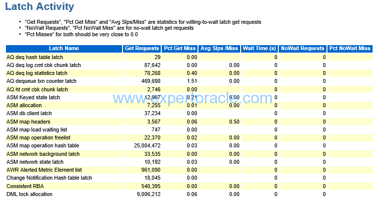
Latch Activity
-
There are a plethora of latch statistics
-
Misses, unless they cause significant amount of sleeps aren’t of concern
-
Sleeps can be a problem
-
May need to look at spin count if you have excessive sleeps
-
Spin count (undocumented (_SPIN_COUNT) was based on CPU speed and 2000 setting was several years ago
-
If latch waits or other latch related events aren’t showing up, then latches probably aren’t an issue
-
Usually cache buffer and shared pool related latches are the major latches.
| PARAMETER | DESCRIPTION | ANALYSIS |
| WAIT TIME (S) | should be 0 | |
| (Pct Get Miss | should be 0 or near 0 |
Segments by Logical Reads

SIGNIFICANCE OF THIS SECTION:
The statistic displays segment details based on logical reads happened. Data displayed is sorted on “Logical Reads” column in descending order. It provides information about segments for which more logical reads are happening. Most of these SQLs can be found under section SQL Statistics -> SQL ordered by Gets.
These reports can help you find objects that are “hot” objects in the database. You may want to review the objects and determine why they are hot, and if there are any tuning opportunities available on those objects (e.g. partitioning), or on SQL accessing those objects.
When the segments are suffering from high logical I/O, those segments are listed here. When the table has high logical reads and its index has relatively small logical reads, there is a high possibility some SQL is using the index inefficiently, which is making a throw-away issue in the table. Find out the columns of the condition evaluated in the table side and move them into the index. When the index has high logical reads, the index is used excessively with wide range. You need to reduce the range with an additional filtering condition whose columns are in the same index.
If a SQL is suboptimal then this can indicate the tables and indexes where the workload or throwaway occurs and where the performance issue lies. It can be particularly useful if there are no actual statistics elsewhere (e.g. Row Source Operation Counts (STAT lines) in the SQL Trace or no actuals in the SQLT/Display Cursor report).
Segments by Physical Reads
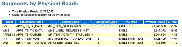
| PARAMETER | DESCRIPTION | ANALYSIS |
| Captured Segments account for 90.8% | This % number is important. It should be high value which shows that we are looking at correct data. |
|
| The top segment record | MTL_ITEM_CATEGORIES | MTL_ITEM_CATEGORIES account for 51.32% of the total physical reads which is a big number. we need to see which SQL statement is using this segment and probably tune that SQL.
You will have to go to “SQL Ordered by Reads” section of AWR to see which SQL Statement is using this segment. |
Segments by Row Lock Waits
Segments by ITL Waits
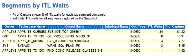
SIGNIFICANCE OF THIS SECTION:
If there is a high level of “enq: TX allocate ITL entry” waits then this section can identify the segments (tables/indexes) on which they occur.
Whenver a transaction modifies segment block, it first add transaction id in the Internal Transaction List table of the block. Size of this table is a block level configurable parameter. Based on the value of this parameter those many ITL slots are created in each block.
ITL wait happens in case total trasactions trying to update same block at the same time are greater than the ITL parameter value.
Total waits happening in the example are very less, 34 is the Max one. Hence it is not recommended to increase the ITL parameter value.
Usually when the segments are suffering from Row Lock, those segments are listed in this section. The general solution is to provide more selective condition for the SQL to lock only rows that are restricted. Or, after DML execution, commit or rollback as soon as possible. Or so on.
Segments by Buffer Busy Waits
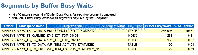
SIGNIFICANCE OF THIS SECTION:
If there is a high level of “Buffer Busy Waits” waits then this section can identify the segments (tables/indexes) on which they occur.
The section lists segments that are suffering from buffer busy waits. Based on the reason code or class#, the treatment of each is different. The physical segment’s attributes such as freelist, freelist groups, pctfree, pctused and so on are handled by rebuilding the object. But before this treatment, you need to check if your SQLs can visit different blocks at the same time if possible to avoid the contention.
Buffer busy waits happen when more than one transaction tries to access same block at the same time. In this scenario, the first transaction which acquires lock on the block will able to proceed further whereas other transaction waits for the first transaction to finish.
If there are more than one instances of a process continuously polling database by executing same SQL (to check if there are any records available for processing), same block is read concurrently by all the instances of a process and this result in Buffer Busy wait event.
This is one of the post in Performance Tuning Fundamentals Series. Click on below links to read more posts from the series:
- Performance Tuning Basics 1 : Selectivity and Cardinality
- Performance Tuning Basics 2 : Parsing
- Performance Tuning Basics 3 : Parent and Child Cursors
- Performance Tuning Basics 4 : Bind Variables
- Performance Tuning Basics 5 : Trace and TKPROF – Part 1: Trace
- Performance Tuning Basics 6 : Trace and TKPROF – Part 2: Generating TKPROF
- Performance Tuning Basics 7 : Trace and TKPROF – Part 3: Analyzing TKPROF Files
- Performance Tuning Basics 8 : Trace File Analyzer (TRCA)
- Performance Tuning Basics 9 : Optimizer Mode
- Performance Tuning Basics 10 : Histograms
- Performance Tuning Basics 11 : Steps to analyze a performance problem
- Performance Tuning Basics 12 : Dynamic Performance Views
- Performance Tuning Basics 13 : Automatic Workload Repository (AWR) Basics
- Performance Tuning Basics 14 : Active Sessions History (ASH) Basics
- Performance Tuning Basics 15 : AWR Report Analysis
- Performance Tuning Basics 16 : Using SQL Tuning Health-Check Script (SQLHC)


- Oracle Multitenant DB 4 : Parameters/SGA/PGA management in CDB-PDB - July 18, 2021
- Oracle Multitenant DB 3 : Data Dictionary Architecture in CDB-PDB - March 20, 2021
- Oracle Multitenant DB 2 : Benefits of the Multitenant Architecture - March 19, 2021
Excellent stuff Brijesh.. 🙂 Really enjoyed reading it…
Hi Brijesh Gogia this is really great work done for you. your research work many people used. Please do and write more Articles AWR report for Solve performance Issue and solutions.
Thanks,
Gowri Infosys India.
Excellent article. Thanks for sharing!
Excellent article. Really liked.
Hi Brijesh,
very Nice article and very help full for new DBA.
Well explained all stuffs.Thanks
Very Good Article. Thanks
Today I learned AWR report in real term. Best way of expalinning
Good article to understand the metrics inside db and it exactly said where to trace.
you are a god
Its too good.If you have any videos on these topics?
Really good information.
This is beyond amazing. Thank you so much for your time in writing this. Very helpful to newcomers.
Excellent
Very detailed and thoughtful. Thanks.
Very useful explained thoroughly.
Hi Sir,
This is Very very helpful for beginners to understand the AWR report
Thanks for the Information.
Excellent,It is what i want
Thank you !!
This very helpful to me
Excellent
Excellent stuff Brijesh !! very informative
Excellent explanation on AWR
Hi Brijesh,
thanks for indeed explanation. I have one query regarding DB cpu utilization .
in your post you have mentioned DBCPU/core* 100. In my case my server have 20core 40 num cpu. CPU distributed to databases on their criticality. one of Database have cpu_count is 19. if I have to calculate CPU utilization for this DB so it would be 19/2=9.5 make it round 10 core or I need to consider cpu_count is core value. in AWR report under load profile DBCPU is 10.38 if I consider core (19/2=9.5 making it round 10 then my database cpu utilization is almost 100%. Could you please explain more on this .
Very good work ..helpful
super post
Good Article and gives sufficient idea on AWR Analysis.
Nice work! Thx!
very good explanation . Thanks alot for sharing
you should have taken a real time example.. or awr with some issue at least
really good article.
Thanks
Really Great work!
Super bien explicado, Muchas gracias!!! =)
Excellent improvement, thank you!
Excelentísimo trabajo de recopilación. Muchísimas gracias.
Thank you Brijesh for writing this. up with great Effort. This is Excellent and no words!